Introduction

This is a short blog post of a series around the importance of writing good code for machine learning and data science projects.

A few months back I answered a question on Quora around suggestions to give to younger data scientists. One of the key points I made was the importance of good coding practices when doing data science and machine learning.

More often I find myself in situations where machine learning and data science projects suffer setbacks because of lack of scalability, general performance issues, lack of testing which presents to re-use the code or bring the models to production.

It seems that for some unknown reasons data scientists have forgotten that software engineering actually matters.

This series aims to bring to the light some these topics.

Writing efficient code for the framework you are using

In the past year I kept track of how often and how I had to fix both my code or someone else code due to performance issues. One thing that came clear is that the first source of poor performance is the lack of understanding of the actual framework or programming language one is using combined with the lack of running any benchmarks on the code. Related to this I also noticed is that the lack of understanding of the framework can often lead to address performance issues in such a way that the code becomes less extensible and maintainable.

Essentially it seems quite hard to find a good balance between writing code that is easy to maintain as well as it performs well.

Here I am going to handcraft a problem similar to something I have seen in a real production environment, to debunk this issue.

A sample simulation engine for random walker

Imagine we need to write a simulation engine for a non-trivial random walk where we have three random walkers which can move forward according to a given probability distribution. We also have a further constraint: every step is randomly shortened according to a different distribution. In short: we have 3 walker c1, c2, c3 and at each step each random walker can move forward of a quantity d which is sampled according to a probability distribution and his journey can be reduced by a certain factor p which is sampled from a different distribution. At each step each walker moves d * p.

This abstract model can be applied to various problems such as predicting the number faulty parts or the dynamic allocation of resources.

For this reason we want to be able to design the engine in such a way that we can dynamically change the two key behaviors:

How much each walker moves forward.
How much the journey of each walker is reduced.

I am going to show you an example written in R to highlight the issue I mentioned at the beginning: the lack of understanding of the framework can lead to bad performances or code that is hard to maintain.

Version 1 i.e. quick and dirty

One quick way to approach the problem is to define a generic function runSim which takes 3 parameters:

The number of steps to simulate n
A function forwardDist which returns a list of 3 numeric values that describe how much each walker will move forward.
A function reductionDist which returns a list of 3 numeric values that describe how much each journey is reduced.

We can write the function runSim to return a matrix n × 3 containing how much the walker will move at each step.

As stated before our initial requirement is to have a generic engine where different forwardDist and reductionDist functions can used.

In the implementation below I am skipping all parameters validation which we should be doing within runSim but for the sake of clarity are not included.

An implementation of runSim could look like this:

runSim <- function(n, forwardDist, reductionDist) {
  simVal <- as.double( replicate(n, Map('*', forwardDist(), reductionDist())))

  matrix(simVal, ncol = 3, byrow = TRUE)
}

Here we made some key design assumptions:

We assumed that forwardDist and reductionDist will return a list of 3 values and the ordering of the two lists is the same. This is necessary so that we can multiply item by item the two list.
We designed forwarDist and reductionDist to return one value for each walker
We use the R replicate to run the simulation n times and the Map function to multiply the two list.

The design seems to meet the original requirement: it allows different forwardDist and reductionDist.

To show how this works we can start with writing a test which implements the forwardDist and reductionDist functions as constant values for each walker.

We call these functions constantForwardDist and constantReductionDist.

constantForwardDist <- function(){
  list(c1=10, c2=30, c3=25)
}

constantReductionDist <- function(){
  list(c1=0.9, c2=0.7, c3=0.1)
}

As you can see the functions return a constant for each walker.

These functions have also a strategic use: they will allow us to run sanity checks in the forms of unit tests around various implementations or versions of runSim. I am using RUnit as framework for unit testing.

library(RUnit)

expectedConstantWalk <-  matrix(rep(c(9, 21, 2.5), 10), ncol = 3, byrow = TRUE)
actualConstantWalk <- runSim(10, constantForwardDist, constantReductionDist)

expectedConstantWalk

##       [,1] [,2] [,3]
##  [1,]    9   21  2.5
##  [2,]    9   21  2.5
##  [3,]    9   21  2.5
##  [4,]    9   21  2.5
##  [5,]    9   21  2.5
##  [6,]    9   21  2.5
##  [7,]    9   21  2.5
##  [8,]    9   21  2.5
##  [9,]    9   21  2.5
## [10,]    9   21  2.5

actualConstantWalk

##       [,1] [,2] [,3]
##  [1,]    9   21  2.5
##  [2,]    9   21  2.5
##  [3,]    9   21  2.5
##  [4,]    9   21  2.5
##  [5,]    9   21  2.5
##  [6,]    9   21  2.5
##  [7,]    9   21  2.5
##  [8,]    9   21  2.5
##  [9,]    9   21  2.5
## [10,]    9   21  2.5

checkEquals(expectedConstantWalk, actualConstantWalk)

## [1] TRUE

At this point we might be quite happy with what we have and we might decide to move on and without doing any benchmarks we might try to implement more complex forwardDist and reductionDist functions.

We start defining non-constant functions for forwardDist which we call normalForwardDist where the forward movements are sampled according to a normal distribution. Each walker is subject to different parameters of the distributions.

normalForwardDist <- function(){
  list(
       c1=rnorm(mean=10, sd=0.5, n=1), 
       c2=rnorm(mean=30, sd=0.5, n=1), 
       c3=rnorm(mean=25, sd=0.5, n=1)
      )
}

The figure below shows the 3 normal distributions used in normalFowardDist.

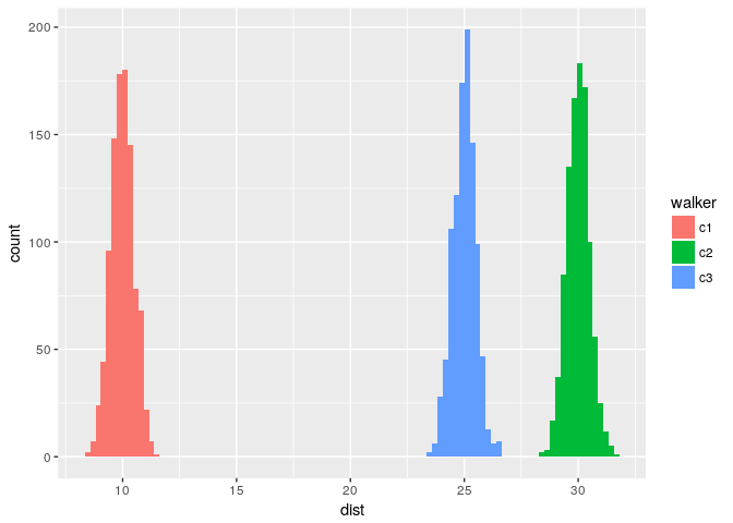
Histogram normal distribution

We can call normalFowardDist very easily to check that everything works as expected:

runSim(10, normalForwardDist, constantReductionDist)

##           [,1]     [,2]     [,3]
##  [1,] 8.796548 20.70411 2.525997
##  [2,] 9.129752 20.92412 2.492297
##  [3,] 8.143187 20.88580 2.537238
##  [4,] 8.922990 21.15933 2.427785
##  [5,] 9.516422 20.32564 2.416143
##  [6,] 8.903545 21.33803 2.472923
##  [7,] 9.283903 20.80704 2.558777
##  [8,] 8.721221 21.30778 2.561612
##  [9,] 8.948482 21.45228 2.490752
## [10,] 8.927771 21.44081 2.540795

Our implementation seems sound: we can customize the logic inside our input functions and we do not need to touch the engine. We have a generic engine. However, when we start plugging large number of $n \approx 10^5$ we notice that the simulation is quite slow: around 2 seconds to generate the walk for just 3 walkers.

We did not run neither profiling nor benchmarks, in a real scenario we could have deployed the engine into production and we just realised it does not scale at all.

We can check how long it takes to compute a walk with $10^5$ steps pretty easily:

system.time(runSim(1e5, normalForwardDist, constantReductionDist))

##    user  system elapsed 
##   2.381   0.007   2.396

Version 2 - a less dirty approach

We need to improve the performance but we do not want to loose flexibility. After all, our initial engine is pretty flexible: we can plug any distribution function to it, and we do not need need to touch it.

Before we start refactoring for performance it is a good idea to have some test that will assure us that the new version behaves like the previous one, when possible,

To do this we generate 1 random walk with the normal distribution function.

set.seed(42)
normalFowrardWalk42 <- runSim(1, normalForwardDist, constantReductionDist)

The first thing we notice is that in runSim we are calling forwardDist and reductionDist n times. Most people learn that R is much faster at dealing with operation on vectors. We also notice that for rnorm and all random generating functions could easily and faster return n variables rather than 1 at the time (benchmark below).

library(rbenchmark)
benchmark( repeatN=rep(rnorm(10, 0.5), 1e6),
           returnN=rnorm(10, 0.5, 1e6)
          )

##      test replications elapsed relative user.self sys.self user.child
## 1 repeatN          100   1.526       NA      1.52        0          0
## 2 returnN          100   0.000       NA      0.00        0          0
##   sys.child
## 1         0
## 2         0

By knowing our framework a little bit better we can rewrite an version of runSim to take advantage of vector-generating functions.

runSim <- function(n, forwardDist, reductionDist) {
  simVal <- as.double(unlist(Map('*', forwardDist(n), reductionDist(n))))
  matrix(simVal, ncol = 3)
}

Note that we need to make a few change inside the function including passing n to forwardDist and reductionDist. This by doing so we have changed the signature of forwardDist and reductionDist and therefore we need to rewrite them again

We start to rewrite our constant ones after all we want to test that this refactoring process is not going to impacting the actual result.

constantForwardDist <- function(n){
  list(c1=rep(10,n), c2=rep(30,n), c3=rep(25,n))
}

constantReductionDist <- function(n){
  list(c1=rep(0.9,n), c2=rep(0.7,n), c3=rep(0.1,n))
}

We run our tests to make sure we did not break anything

checkEquals(expectedConstantWalk, runSim(10, constantForwardDist, constantReductionDist)) 

## [1] TRUE

and now we can proceed rewriting normalForwardDist as

normalForwardDist <- function(n){
  list(
       c1=rnorm(mean=10, sd=0.5, n=n), 
       c2=rnorm(mean=30, sd=0.5, n=n), 
       c3=rnorm(mean=25, sd=0.5, n=n)
      )
}

as sanity check we can reset the random seed and compare that the new version of normalForwardDist returns the same result which we have stored normalFowrardWalk42.

set.seed(42)
acutalForwardNormal <- runSim(1, normalForwardDist, constantReductionDist)
checkEquals( normalFowrardWalk42, acutalForwardNormal)

## [1] TRUE

# We store this for further tests
set.seed(42)
normalFowrardWalk42e2 <- runSim(100, normalForwardDist, constantReductionDist)

Further steps of the walk will be different as the in the first approach we generate 1 random variate at the time for each walker, whereas, in the second approach we generate n variate for each walker at one time.

Now the question is how faster is this approach compared the previous one: what improvement did we make? We can run a simple benchmark test with various size of the simulation compute how long it takes to execute the full walk. To run the benchmark I am using Rbenchmark and I set 50 repetitions for each walk to average the execution times. The average execution time for the two version is displayed below.

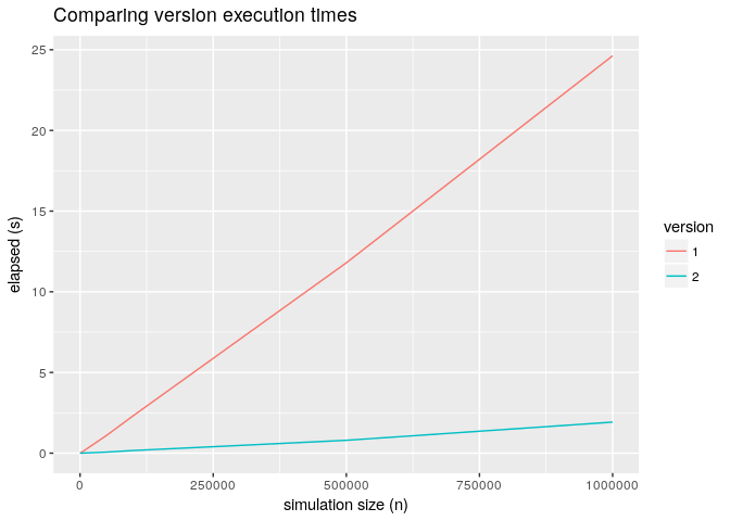
Execution comparisons

We made a substantial improvement and for large n version 2 is 10x faster.

Version 3 - how fast can we go without any flexibility.

We could stop here but out of curiosity we want to understand if we can make further improvements by writing a specific simulation engine for the normal distribution problem.

We want to answer the following question: how much performance do we need to trade off in exchange for flexibility ?

An inflexible but quite efficient way to write runSim for the normal distribution is to hard-code the function inside runSim:

runSim <- function(n) {
  
  simVal <- c( rnorm(mean=10, sd=0.5, n=n) * 0.9, 
               rnorm(mean=30, sd=0.5, n=n) * 0.7, 
               rnorm(mean=25, sd=0.5, n=n)* 0.1  
            )
  
  matrix(simVal, ncol = 3)
}

This implementation of runSim is missing all the flexibility of our previous version. We need to implement a version of runSim for each distribution and it only supports 3 walkers. But we do not really care as the goal is to understand what is the trade-off we are paying.

As we did before we test that we are getting the same results, we need to make sure we are comparing apples to apples! This approach should return the same result as our second version even for n > 1.

set.seed(42)
actualNormalWalk <- runSim(100)

checkEquals(normalFowrardWalk42e2, actualNormalWalk)

## [1] TRUE

Now we can answer our question is how much faster is this version 3 compared to version 2. Below the result of a benchmark:

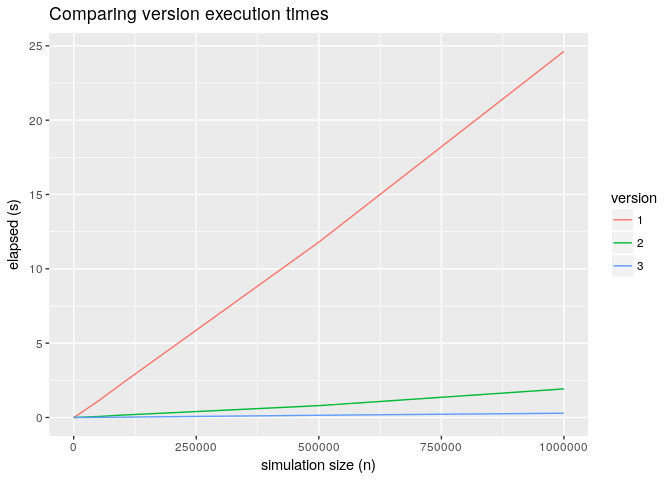
Execution comparisons version 2 and version 3

The previous graph is not very comforting the trade off between performance and flexibility is close to 10x for large values of n.

At this point I witnessed people in production settings going for the ugly, hardly re-usable and quite hard to maintain solution.

Version 4 – I don’t like pigs with lipsticks

But do we really need to stop to version 2 or version 3?

It turns out that if we spend some time understanding how the framework we are using works and we start profiling the code we could try to make so important changes.

For example we can rewrite forwardDist and reductionDist in a slightly different way.

Instead of returning a numeric value for each walker we can return functions.

constantForwardDist <- function(){
  list(
       c1=function(n){rep(10,n)}, 
       c2=function(n){rep(30,n)}, 
       c3=function(n){rep(25,n)}
      )
}

constantReductionDist <- function(){
  list(
       c1=function(n){rep(0.9,n)}, 
       c2=function(n){rep(0.7,n)}, 
       c3=function(n){rep(0.1,n)}
      )
}


normalForwardDist <- function(){
  list(
       c1=function(n){rnorm(mean=10, sd=0.5, n=n)}, 
       c2=function(n){rnorm(mean=30, sd=0.5, n=n)}, 
       c3=function(n){rnorm(mean=25, sd=0.5, n=n)}
       )
}

The difference with this approach is that when we call the function instead of a list of size 3 containing 3 vectors of size n we get a list of size 3 containing 3 functions.

normalForwardDist()

## $c1
## function (n) 
## {
##     rnorm(mean = 10, sd = 0.5, n = n)
## }
## <environment: 0x55c615af85a0>
## 
## $c2
## function (n) 
## {
##     rnorm(mean = 30, sd = 0.5, n = n)
## }
## <environment: 0x55c615af85a0>
## 
## $c3
## function (n) 
## {
##     rnorm(mean = 25, sd = 0.5, n = n)
## }
## <environment: 0x55c615af85a0>

We can also start to think about rewriting runSim to work with and arbitrary number of walkers and for good measure we might also match the forwardDist and reductionDist walkers, that is forwe don’t need to force ordering in the forwardDist and reductionDist functions which is a big plus when multiple people might end up writing these functions.

Our new version of runSim would look like this

runSim <- function(n, forwardDist, reductionDist, walkers=c("c1", "c2", "c3")) {
  
  simValMatix <- vapply(walkers, function(walker) {
      walkerForwardDist <- forwardDist()[[walker]]
      walkerReductionDist <- reductionDist()[[walker]]
      walkerForwardDist(n) * walkerReductionDist(n)
  }, rep(0.0, n), USE.NAMES = FALSE)
  
  simValMatix
}

Note that I used vapply and anonymous functions. I also tested a similar version with for loops and pre-allocation of the memory which had similar performance. I settle down for the vapply variant as O found it easier to read.

Also in vapply we set USE.NAMES = FALSE to make sure that the result matches exactly the previous one.

This last step is necessary if we want to keep the return value of runSim consistent with the previous versions, which often required when you start to refactor a large project.

As per usual we run our tests: first against the constant functions

actualConstantWalk <- runSim(10, constantForwardDist, constantReductionDist, walkers = c("c1", "c2", "c3"))
checkEquals(expectedConstantWalk, actualConstantWalk)

## [1] TRUE

and the against the normalForwardDist

set.seed(42)
actualNormalWalk <- runSim(100, normalForwardDist, constantReductionDist, walkers = c("c1", "c2", "c3"))
checkEquals(normalFowrardWalk42e2, actualNormalWalk)

## [1] TRUE

We are happy that the refactor did not impact the result of the simulation but the big question is are we getting better comparable performance to version 3?

Below the picture of a benchmark that shows the various versions and zooms into the
version 3 vs version 4.

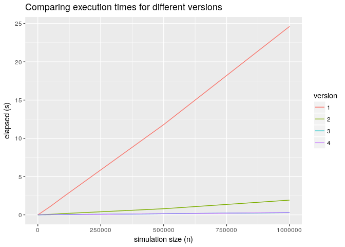
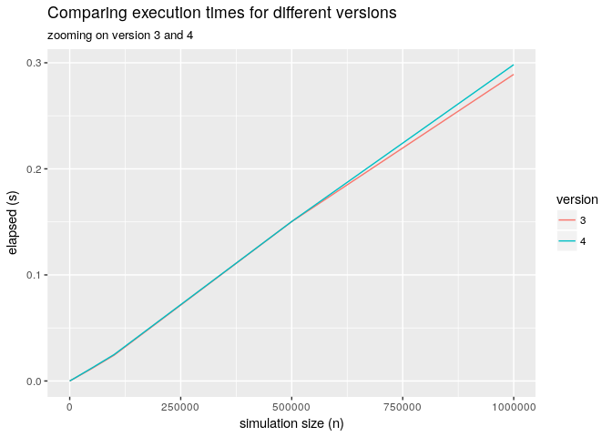
Execution comparisons

As you can see from the graph above the overhead of the more flexible implementation is pretty much negligible.

The two key conclusions from this short article are:

A good understanding of the framework you use will help you to optimize your code.
You must have unit tests in order to be able to start any refactor effectively.
Quite often you do not need to trade off flexibility to performance.